Spatially Periodic Reaction-Diffusion Equations

A mathematical survey of persistence, pulsating fronts, spreading geometry, and large-time profiles in periodic environments.

Starting from fragmented-habitat models, we follow the questions they generate: when does a population persist, which fronts exist, what determines their speeds, and which profiles emerge from the Cauchy problem? Results are stated without proofs, with hypotheses and references. The main setting is a scalar local reaction–diffusion equation; extensions to periodic domains, interface conditions, space–time periodicity, and multistability are developed in Sections 7–8.

Literature updated: October 2026. General perspectives: Xin [48]; Hamel–Rossi [49].

1. Background and Biological Motivation

Let \(u(t,x)\) denote population density. The model of Shigesada, Kawasaki and Teramoto [1] combines Fickian dispersal, spatially varying low-density growth, and intraspecific competition in a periodically fragmented habitat.

The homogeneous starting point is the Fisher–KPP equation [12], [13], \(u_t=D\Delta u+ru(1-u)\), with minimal planar speed \(2\sqrt{Dr}\). Aronson–Weinberger [14] connected traveling fronts to the large-time spreading of localized populations. Spatial fragmentation replaces a constant growth rate by a periodic environment and turns this speed-selection problem into a spectral and geometric one.

1.1. A One-Dimensional Patch Model

In the 1986 model [1], the population satisfies

\[ \partial_t u(t,x) = \partial_x\!\left(D(x)\partial_x u(t,x)\right) + \bigl(r(x)-\mu u(t,x)\bigr)u(t,x), \qquad t>0,\quad x\in\mathbb R,\quad \mu>0. \tag{B1} \]

Dispersal

\(\partial_x(D(x)\partial_x u)\)

Fickian movement with patch-dependent diffusivity \(D_i>0\); the flux matches across patch boundaries.

Low-density growth

\(r(x)u\)

Positive \(r_i\) means growth when the population is rare; negative \(r_i\) means local decline.

Intraspecific competition

\(-\mu u^2,\quad\mu>0\)

A density-dependent loss in both patch types, independent of the sign of \(r_i\).

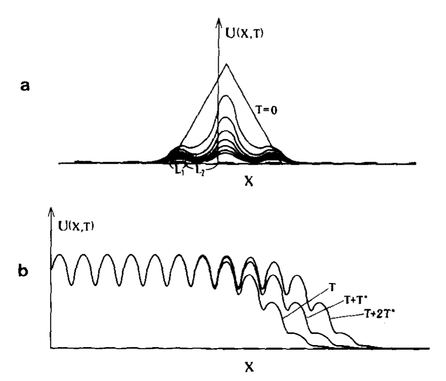
The competition coefficient \(\mu>0\) is constant. Let \(D_1,D_2>0\), \(r_1\geq r_2\), \(r_1>0\), and let \(L_1,L_2>0\) be the widths of the two patch types. One habitat period has length \(L=L_1+L_2\). The coefficients are

\[ (D(x),r(x))= \begin{cases} (D_1,r_1),&kL<x<kL+L_1,\\ (D_2,r_2),&kL+L_1<x<(k+1)L, \end{cases} \qquad k\in\mathbb Z. \tag{B2} \]

The coefficients repeat every \(L\). At each interface \(x_j\in\{kL,kL+L_1:k\in\mathbb Z\}\), density and flux are continuous:

\[ [u]_{x_j}=0,\qquad [D u_x]_{x_j}=0, \qquad [h]_{x_j}:=h(x_j^+)-h(x_j^-). \tag{B3} \]

Jump notation. The brackets \([h]_{x_j}\) measure the jump of \(h\) across the interface \(x_j\): \(h(x_j^+)\) is the limit from the right and \(h(x_j^-)\) is the limit from the left. The subscript identifies the interface; it does not indicate differentiation.

Thus \([u]_{x_j}=0\) means that population density has the same value on both sides, and \([D u_x]_{x_j}=0\) means that the diffusion flux matches across the interface [1]. Derivatives are taken inside each patch. When \(D\) changes at an interface, the slopes \(u_x\) on the two sides may differ while \(D u_x\) remains continuous.

In the interiors of the patches, (B1) reads \(u_t=D_i u_{xx}+r_i u-\mu u^2\). The initial population in [1] is continuous, nonnegative, single-peaked, and confined to a bounded interval:

\[ u(0,x)=u_0(x)\geq0,\qquad u_0\not\equiv0, \qquad \operatorname{supp}u_0\subset[-R,R],\quad R>0. \tag{B4} \]

The central question · Shigesada–Kawasaki–Teramoto (1986) [1]

When does a species invade a periodically fragmented habitat, and when does it become extinct?

How are the outcome and propagation speed determined by \(L_1,L_2,D_1,D_2,r_1,r_2\)? The alternating habitat is illustrated in Figure 1.

Figure 1. Schematic of the one-dimensional periodic habitat in (B2), motivated by [1]. The widths of the two patch types are \(L_1\) and \(L_2\).

Analytical result · Linear invasion threshold [1]

For (B1)–(B3), assume \(r_1>0>r_2\). Define

\[ L_{1,\mathrm{crit}} =2\sqrt{\frac{D_1}{r_1}}\, \arctan\!\left[ \sqrt{\frac{-r_2D_2}{r_1D_1}}\, \tanh\!\left(\frac{L_2}{2}\sqrt{\frac{-r_2}{D_2}}\right) \right]. \tag{B5} \]

The linearization \(v_t=(D(x)v_x)_x+r(x)v\), with the same interface conditions, satisfies the following stability criterion at \(v\equiv0\):

\[ \begin{aligned} L_1<L_{1,\mathrm{crit}} &\ \Longrightarrow\ v\equiv0\ \text{is linearly stable},\\[1mm] L_1>L_{1,\mathrm{crit}} &\ \Longrightarrow\ v\equiv0\ \text{is linearly unstable}. \end{aligned} \tag{B6} \]

Source: [1]. The equality \(L_1=L_{1,\mathrm{crit}}\) defines the critical boundary.

The threshold tests growth from a rare population. Persistence of a positive periodic state and nonlinear spreading are the subsequent questions addressed in §§2.3–6.

Periodic invaded state and traveling periodic wave

The positive stationary state considered in [1], when it exists, is a periodic function \(p\):

\[ \begin{cases} (D(x)p')'+\bigl(r(x)-\mu p\bigr)p=0 &\text{inside each patch},\\ p(x+L)=p(x)>0,\\ [p]_{x_j}=[Dp']_{x_j}=0. \end{cases} \tag{B7} \]

For a right-moving traveling periodic wave (TPW), the formulation in [1] becomes

\[ \begin{gathered} u_{\mathrm{TPW}}(t+T,x+L)=u_{\mathrm{TPW}}(t,x), \qquad T>0,\qquad c=\frac{L}{T},\\ \lim_{x\to+\infty}u_{\mathrm{TPW}}(t,x)=0,\qquad \lim_{x\to-\infty}\bigl(u_{\mathrm{TPW}}(t,x)-p(x)\bigr)=0. \end{gathered} \tag{B8} \]

Numerical observations in the 1986 paper

For the localized initial distributions studied in [1], the computations report extinction on the linearly stable side and outward spreading in both directions on the unstable side. In the spreading case, the profiles approach the TPW pattern, while the population near the introduction site approaches a periodic stationary distribution.

Original numerical simulations: (a) population profiles decay to extinction; (b) a traveling periodic wave on the positive half-axis at times T, T+T*, and T+2T*. — **Numerical simulations.** (a) Extinction from a localized initial population. (b) A traveling periodic wave at successive times. Source: [1].

Leading-edge dispersion relation

Purpose: estimating the invasion speed. Once an invasion can establish, the next question is how fast its front moves. The paper studies the low-density leading edge, where the competition term is small and the linearized equation provides a speed relation. Seek a leading edge of the form

\[ v(t,x)=e^{-\sigma(x-ct)}g(x),\qquad \sigma>0,\qquad g(x+L)=g(x)>0, \qquad [g]_{x_j}=[D(g'-\sigma g)]_{x_j}=0. \tag{B9} \]

Here \(c\) is the propagation speed, \(\sigma\) is the exponential decay rate ahead of the front, and \(g(x)\) describes the modulation caused by the periodic habitat. A larger \(\sigma\) means a more rapidly decaying leading-edge envelope.

The solutions in the two patch types must join with continuous density and flux and satisfy the periodicity of \(g\). These requirements impose a compatibility condition between \(c\) and \(\sigma\), called the dispersion relation [1]:

\[ \cosh(\sigma L)=\cosh(q_1L_1)\cosh(q_2L_2)+\frac{(D_1q_1)^2+(D_2q_2)^2}{2D_1D_2q_1q_2}\sinh(q_1L_1)\sinh(q_2L_2). \tag{B10} \]

\(q_i^2=(c\sigma-r_i)/D_i\), \(i=1,2\). In (B10), \(D_i,r_i,L_i\) are the given habitat parameters. The quantities \(q_i\) are auxiliary quantities determined by \(c\) and \(\sigma\). The left-hand side describes exponential decay across one habitat period; the right-hand side combines the two patch solutions and their interface conditions. Equality means that the proposed speed and decay rate are compatible with the periodic habitat.

How to use (B10).

Fix the habitat parameters and choose a decay rate \(\sigma>0\). Solve (B10) for \(c\), retaining the branch with a positive periodic profile \(g\).
Vary \(\sigma\) to obtain the speed curve \(c=c(\sigma)\). Its lowest value gives the minimum leading-edge speed:

\[ c_{\min}=\min_{\sigma>0}c(\sigma). \tag{B11} \]

If \(q_i\) is imaginary, the admissible branch must satisfy \(|q_i|L_i\leq\pi\), and the hyperbolic factors are evaluated using their trigonometric counterparts. At \(q_i=0\), the expression is understood by continuity.

Thus (B10)–(B11) turn the habitat parameters into a computable candidate for the invasion speed. The nonlinear simulations in [1] approach this minimum.

Mathematical question · Spreading speed and front convergence

Consider (B1)–(B3) [1] in the invasion regime \(r_1>0>r_2\) and \(L_1>L_{1,\mathrm{crit}}\). Let \(p(x)>0\) be the periodic stationary state, and let \(u(t,x)\) start from any continuous, compactly supported initial population \(u_0\geq0\), \(u_0\not\equiv0\).

1. Does the nonlinear invasion select the speed \(c_{\min}\) computed in (B10)–(B11)? More precisely, do the following limits hold?

\[ \begin{aligned} \lim_{t\to\infty}\ \sup_{|x|\leq ct}|u(t,x)-p(x)|&=0, &&0<c<c_{\min},\\[1mm] \lim_{t\to\infty}\ \sup_{|x|\geq ct}u(t,x)&=0, &&c>c_{\min}. \end{aligned} \]

The first limit means that the population settles to \(p(x)\) throughout every region expanding slower than \(c_{\min}\). The second means that the density tends to zero beyond every region expanding faster than \(c_{\min}\).

2. Does the spreading front approach a traveling periodic wave? Is there a right-moving TPW \(U_*(t,x)=\Phi_*(x,x-c_{\min}t)\) of (B1)–(B3), with periodic profile \(\Phi_*(x+L,z)=\Phi_*(x,z)\), connecting \(p(x)\) behind the front to \(0\) ahead, and a front position \(m(t)=c_{\min}t+o(t)\), such that for every fixed \(R>0\),

\[ \lim_{t\to\infty}\ \sup_{|z|\leq R}\left|u(t,m(t)+z)-\Phi_*(m(t)+z,z)\right|=0? \]

This asks whether the solution near the moving front approaches the TPW profile. The correction \(m(t)-c_{\min}t=o(t)\) allows a possible delay while keeping the asymptotic speed equal to \(c_{\min}\). The corresponding convergence question is also posed for the left-moving front.

Connection with the later sections. The patch model separates three questions: the linear invasion threshold, the construction and speed of a periodic front, and the long-time behavior of an initially localized population. These distinctions organize the discussion of pulsating fronts, front speeds, and the Cauchy problem below.

1.2. Two-Dimensional Stripes and Anisotropic Spreading

Striped habitat model, motivated by Kinezaki et al. [6]:

\[ u_t=\nabla_{x,y}\cdot\!\left(D(x)\nabla_{x,y}u\right)+(r(x)-\mu u)u, \quad (x,y)\in\mathbb R^2,\quad t>0. \tag{B12} \]

\[ D(x+L)=D(x)>0,\quad r(x+L)=r(x),\quad\mu>0, \qquad e_\vartheta=(\cos\vartheta,\sin\vartheta). \]

Two initial-data geometries:

\[ \begin{array}{ll} \text{Strip introduction:}&u_0(x,y)=g((x,y)\cdot e),\quad 0\leq g\in C_c(\mathbb R),\quad g\not\equiv0,\\ \text{Localized introduction:}&0\leq u_0\in C_c(\mathbb R^2),\quad u_0\not\equiv0. \end{array} \tag{B13} \]

Mathematical question · Direction and shape

For localized data in an invasion regime, determine \(w(\vartheta)\) and \(W\):

\[ \begin{gathered} u(t,ct e_\vartheta)-p(ct\cos\vartheta)\longrightarrow0 \quad(0\leq c<w(\vartheta)),\\ u(t,ct e_\vartheta)\longrightarrow0\quad(c>w(\vartheta)),\\ W=\{r e_\vartheta:0\leq r<w(\vartheta),\ 0\leq\vartheta<2\pi\}. \end{gathered} \]

Here \(p(x)>0\) is the periodic invaded state. How do \(D_i,r_i,L_i\) determine \(w\) and \(\partial W\)?

Reported patterns [6]: nearly circular, oval, or spindle-shaped; elongated along the stripes in the configurations studied.

Figure 2. Anisotropic spreading in a periodically striped habitat. Schematic: direction-dependent spread, elongated parallel to the stripes [6].

1.3. From Patch Models to Periodic Operators

\[ \underbrace{u_t}_{\text{density change}}=\underbrace{\nabla\cdot(A(x)\nabla u)}_{\text{diffusion}}+\underbrace{b(x)\cdot\nabla u}_{\text{drift}}+\underbrace{f(x,u)}_{\text{reaction}}. \]

Patch model: \(N=1\), \(A=D\), \(b=0\), \(f(x,s)=(r(x)-\mu s)s\). Its invaded state is \(p(x)\); Sections 2–5 use equilibria \(0\) and \(1\), except where \(p(x)\) is specified.

Figure 3. Front geometry: invaded state behind; low density ahead. In periodic media, \(u(t,x)=\Phi(x,x\cdot e-ct)\).

2. Equation, Assumptions, and Reaction Classes

2.1. Periodic equation

\[ u_t=\mathcal A u+f(x,u),\qquad \mathcal A u:=\nabla\cdot(A(x)\nabla u)+b(x)\cdot\nabla u, \quad (t,x)\in I\times\mathbb R^N. \tag{1} \]

\(I=(0,\infty)\) for the Cauchy problem; \(I=\mathbb R\) for an entire front.

(H1) Periodicity and regularity. Fix \(\alpha\in(0,1)\), \(\ell_i>0\), and

\[ \begin{gathered} Q=\prod_{i=1}^N(0,\ell_i),\qquad \mathcal L=\ell_1\mathbb Z\times\cdots\times\ell_N\mathbb Z,\\ A\in C^{2,\alpha},\quad b\in C^{1,\alpha},\quad f,\ f_s\in C^{0,\alpha}(\mathbb R^N\times[0,1]),\\ A(x+k)=A(x),\quad b(x+k)=b(x),\quad f(x+k,s)=f(x,s)\quad(k\in\mathcal L). \end{gathered} \]

(H2) Uniform ellipticity.

\[ A(x)=A(x)^{\mathsf T},\qquad 0<\lambda_0|\eta|^2\leq\eta\cdot A(x)\eta\leq\Lambda_0|\eta|^2 \quad(\eta\neq0). \]

(H3) Incompressible flow with zero mean.

\[ \nabla\cdot b=0,\qquad \int_Q b(x)\,dx=0. \]

(H4) Equilibria.

\[ f(x,0)=f(x,1)=0,\qquad 0\leq u_0\leq1\ \Longrightarrow\ 0\leq u(t,\cdot)\leq1. \]

These are the baseline hypotheses for the normalized smooth equation. Subsections with a periodic invaded state, a changing-sign growth rate, boundary or interface conditions, or time-dependent coefficients state their own setting. In particular, (H3) is a restriction on the flow, rather than a general property of periodic advection.

2.2. Three reaction classes

(K) Fisher–KPP.

\[ a(x):=f_s(x,0)>0,\qquad 0<f(x,s)\leq a(x)s\quad(0<s<1). \tag{K} \]

(I) Ignition. For some \(\theta\in(0,1)\), \(\delta\in(0,1-\theta)\),

\[ f(x,s)=0\ (0\leq s\leq\theta),\qquad f(x,s)>0\ (\theta<s<1),\qquad f_s(x,s)\leq0\ (1-\delta\leq s\leq1). \tag{I} \]

(B) Bistable. For a periodic threshold \(\theta(x)\in(0,1)\) and \(\gamma>0\),

\[ \begin{gathered} f(x,\theta(x))=0,\qquad \begin{cases} f(x,s)<0,&0<s<\theta(x),\\ f(x,s)>0,&\theta(x)<s<1, \end{cases}\\ f_s(x,0)\leq-\gamma,\qquad f_s(x,1)\leq-\gamma. \end{gathered} \tag{B} \]

Reaction profiles at a fixed \(x\), shown schematically. Teal: \(f>0\); brown: \(f<0\).

2.3. Persistence before propagation

Hostile patches allow negative local growth. A useful unnormalized model is

\[u_t=\nabla\cdot(A(x)\nabla u)+r(x)u-\beta(x)u^2,\qquad b=0,\quad \beta(x)\geq\beta_0>0.\]

Here \(A,r,\beta\) are smooth and periodic, \(A\) is uniformly elliptic, and \(r\) may change sign. Define the principal growth eigenvalue by

\[\nabla\cdot(A\nabla\varphi)+r(x)\varphi=\kappa\varphi,\qquad \varphi>0,\quad\varphi\text{ periodic}.\]

Persistence criterion · Berestycki–Hamel–Roques [18]. For nonzero, nonnegative, bounded, continuous initial data,

\[\kappa\leq0\ \Longrightarrow\ \|u(t,\cdot)\|_\infty\to0,\qquad \kappa>0\ \Longrightarrow\ u(t,\cdot)\to p\text{ locally uniformly}.\]

In the second case, \(p\) is the unique positive periodic equilibrium. The threshold depends on the whole cell and its diffusion, rather than only on the sign of \(r\) in an individual patch.

The eigenvalue and maximum-principle framework is developed by Berestycki–Nirenberg–Varadhan [19] and, for unbounded domains and generalized principal eigenvalues, Berestycki–Rossi [20]. The periodic criterion above gives a rigorous counterpart to the invasion threshold in §1.1; fronts connecting \(p(x)\) to \(0\) belong to the theory in [5].

3. Pulsating Traveling Fronts

3.1. Definition and existence question

Definition. A front in direction \(e\in\mathbb S^{N-1}\), with speed \(c\in\mathbb R\setminus\{0\}\), is an entire solution of (1) satisfying

\[ \begin{gathered} u(t,x)=\Phi(x,z),\qquad z=x\cdot e-ct,\qquad 0<\Phi<1,\\ \Phi(x+k,z)=\Phi(x,z)\quad(k\in\mathcal L),\\ \lim_{z\to-\infty}\sup_{x\in Q}|\Phi(x,z)-1|=0,\qquad \lim_{z\to+\infty}\sup_{x\in Q}\Phi(x,z)=0. \end{gathered} \tag{2} \]

\(z\to-\infty\): invaded side; \(z\to+\infty\): leading edge. Positive speed means propagation toward \(e\); negative speed means retreat in that orientation. A stationary connection is treated separately. Monotonicity of the profile is included in the results below.

Mathematical question · Admissible speeds

For fixed \((A,b,f,e)\), determine

\[ \mathscr C(e):=\{c>0:\text{a front satisfying (1)–(2) exists}\}. \tag{3} \]

Is \(\mathscr C(e)\) empty, a singleton, or an interval? Is the profile unique up to \(z\)-translation?

3.2. Ignition: one speed

Theorem 1 · Berestycki–Hamel [3]. Assume (H1)–(H4) and (I). Then, for every \(e\in\mathbb S^{N-1}\),

\[ \exists\,c_I(e)>0:\qquad \mathscr C(e)=\{c_I(e)\},\qquad \Phi_z<0. \tag{4} \]

Any two front profiles \(\Phi_1,\Phi_2\) in direction \(e\) satisfy

\[ \exists\tau\in\mathbb R:\qquad \Phi_2(x,z)=\Phi_1(x,z+\tau). \]

3.3. KPP and monostable reactions: a speed threshold

Theorem 2 · Periodic KPP fronts [3], [4]. Assume (H1)–(H4) and (K). Then

\[ \forall e\in\mathbb S^{N-1},\qquad \exists\,c^*(e)>0:\quad \mathscr C(e)=[c^*(e),\infty). \tag{5} \]

The spectral formula for \(c^*(e)\) is given in Section 4.1.

Monostable extension [3]

Under (H1)–(H4), assume \(f_s(x,s)\leq0\) near \(s=1\). Then

\[ f(x,s)>0\quad(0<s<1) \quad\Longrightarrow\quad \mathscr C(e)=[c_M^*(e),\infty),\quad c_M^*(e)>0. \]

The KPP bound \(f(x,s)\leq f_s(x,0)s\) is the additional hypothesis for the linear speed formula.

3.4. Bistable reactions: dependence on the spatial period

Let \(a>0\) and \(f\) be smooth and 1-periodic in \(y\), with \(f\) satisfying (B). Consider

\[ u_t=\partial_x\!\left(a(x/L)u_x\right)+f(x/L,u),\qquad L>0. \tag{6} \]

\(a_H:=\left(\int_0^1 a(y)^{-1}\,dy\right)^{-1}\), \(\bar f(s):=\int_0^1 f(y,s)\,dy\).

Theorem 3 · Ding–Hamel–Zhao [7]. Suppose the homogenized equation has a unique front up to translation:

\[ a_H\phi_0''+c_0\phi_0'+\bar f(\phi_0)=0,\qquad \phi_0(-\infty)=1,\quad\phi_0(+\infty)=0,\quad c_0\neq0. \]

Then, for some \(L_*>0\),

\[ \begin{gathered} 0<L<L_*\ \Longrightarrow\ \exists\,u_L(t,x)=\Phi_L(x/L,x-c_Lt),\qquad c_L\neq0,\\ \Phi_L(y+1,z)=\Phi_L(y,z),\qquad \Phi_L(y,-\infty)=1,\quad\Phi_L(y,+\infty)=0,\\ \lim_{L\to0^+}c_L=c_0. \end{gathered} \]

The front is unique up to a time translation. For large periods, another sufficient condition is

\[ \begin{gathered} \int_0^1 f(y,s)\,ds>0,\quad f_s(y,\theta(y))>0\quad\forall y\\ \Longrightarrow\quad\exists L^*>0:\qquad L>L^*\ \Rightarrow\ \exists\text{ a front with }c_L>0. \end{gathered} \]

Blocking [2]. Periodic bistable media can also admit stationary interfaces and suppress propagation.

Open problem · Propagation or pinning?

\[ \mathcal E(a,f):=\{L>0:\exists\text{ a pulsating front with }c_L\neq0\}. \]

Given \((a,f)\), characterize \(\mathcal E(a,f)\) and its boundary. For which \(L\) does a stationary connection exist?

\[ \partial_x\!\left(a(x/L)p'\right)+f(x/L,p)=0,\quad 0<p<1,\quad p(-\infty)=1,\quad p(+\infty)=0. \]

3.5. Uniqueness, leading edges, and pushed fronts

Qualitative front analysis includes strict monotonicity, decay at the end states, and uniqueness up to a time shift. Hamel [21] derives precise leading-edge asymptotics; Hamel–Roques [22] establish uniqueness and stability under strict KPP and end-state stability hypotheses, including critical fronts with suitable matching conditions on the initial tail.

Linear and nonlinear selection. For a smooth monostable reaction with \(f_s(x,0)>0\), let \(c_M^*(e)\) be the minimal nonlinear front speed and set

\[c_{\mathrm{lin}}(e):=\min_{\sigma>0}\frac{\lambda(e,\sigma)}{\sigma},\qquad c_M^*(e)\geq c_{\mathrm{lin}}(e).\]

The KPP inequality gives equality. A minimal front is called pushed when \(c_M^*(e)>c_{\mathrm{lin}}(e)\). Guo [23] studies the leading-edge decay and stability of pushed pulsating fronts. Consequently, the eigenvalue formula in §4 is specific to linear determinacy.

3.6. Bistable existence, counterexamples, and terraces

Fang–Zhao [24] provide an existence framework for bistable traveling waves of monotone semiflows, including periodic problems, under their counter-propagation and compactness hypotheses. In contrast, Zlatoš [25] constructs periodic bistable reactions without a transition front. Thus the pointwise sign pattern (B) alone is insufficient to guarantee a single front connecting \(1\) to \(0\).

Ding–Hamel–Zhao [7] resolve existence and stability in several spatial-period regimes. Ding–Hamel–Liang [26] determine the large-period speed under uniformly favorable frozen bistable dynamics; the limit is stated in §7.1. Giletti–Rossi [43] develop the multidimensional multistable theory, where intermediate periodic states can produce a propagating terrace (§8.2).

4. Minimal Speeds and Spectral Problems

Mathematical question · Linear determinacy

For (H1)–(H4) and (K), can the nonlinear front speed be recovered from the linearization at \(u=0\)?

\[ v_t=\mathcal A v+a(x)v,\qquad v(t,x)=e^{-\sigma(x\cdot e-ct)}\varphi(x),\quad \sigma>0. \]

4.1. Periodic principal eigenvalue

Set \(\mathcal L_0:=\mathcal A+a(x)\). Exponential conjugation gives

\[ \begin{aligned} \mathcal L_{e,\sigma}\varphi&:=e^{\sigma x\cdot e}\mathcal L_0\!\left(e^{-\sigma x\cdot e}\varphi\right)\\ &=\nabla\cdot(A\nabla\varphi)+(b-2\sigma Ae)\cdot\nabla\varphi+\left[\sigma^2e\cdot Ae-\sigma\nabla\cdot(Ae)-\sigma b\cdot e+a(x)\right]\varphi. \end{aligned} \tag{7} \]

Principal eigenpair.

\[ \begin{cases} \mathcal L_{e,\sigma}\varphi_{e,\sigma} =\lambda(e,\sigma)\varphi_{e,\sigma}&\text{in }\mathbb R^N,\\ \varphi_{e,\sigma}>0,\qquad \varphi_{e,\sigma}(x+k)=\varphi_{e,\sigma}(x)&k\in\mathcal L,\\ \displaystyle\int_Q\varphi_{e,\sigma}^2\,dx=1. \end{cases} \]

Theorem 4 · Berestycki–Hamel–Nadirashvili [4]. Under (H1)–(H4) and (K),

\[ c^*(e)=\min_{\sigma>0}\frac{\lambda(e,\sigma)}{\sigma}. \tag{8} \]

Here \(\sigma\) is the exponential decay rate, and \(\lambda(e,\sigma)/\sigma\) is the speed of the corresponding linear mode.

4.2. Homogeneous check

For \(A=D I_N\), \(b=0\), \(a(x)=r>0\),

\[ \lambda(e,\sigma)=D\sigma^2+r,\qquad c^*=\min_{\sigma>0}\left(D\sigma+\frac r\sigma\right) =2\sqrt{Dr},\qquad \sigma_* =\sqrt{r/D}. \]

4.3. Periodic invaded states

Biological invasion model [5]

For periodic KPP models with a positive periodic invaded state \(p\), the front connects \(p(x)\) to \(0\):

\[ \mathcal A p+f(x,p)=0,\quad p(x+k)=p(x)>0,\qquad \Phi(x,-\infty)=p(x),\quad \Phi(x,+\infty)=0. \]

The linear operator at \(0\) remains \(\mathcal A+f_s(x,0)\).

4.4. Beyond the linear spectral formula

For ignition and general monostable reactions, El Smaily [27] gives nonlinear min–max descriptions of front speeds. A useful profile operator, with \(D_e=\nabla_x+e\partial_z\), is

\[\mathcal P_e\Phi:=D_e\cdot(A(x)D_e\Phi)+b(x)\cdot D_e\Phi+f(x,\Phi),\qquad c=-\frac{\mathcal P_e\Phi}{\Phi_z}.\]

The last identity holds for an actual strictly decreasing front. The variational theory optimizes corresponding quotients over admissible profiles with the prescribed periodicity and end states. It retains the full nonlinearity, which is essential for ignition and pushed fronts.

Weinberger [16] and Liang–Zhao [17] place spreading speeds and traveling waves in an order-preserving evolution framework. This connects PDE results with periodic recursions and monotone semiflows, under their respective comparison, compactness, and monostability assumptions.

5. Cauchy Problems and Spreading Geometry

5.1. Compact initial populations

\[ \begin{cases} u_t=\mathcal A u+f(x,u),&t>0,\quad x\in\mathbb R^N,\\ u(0,x)=u_0(x),&0\leq u_0\leq1,\quad u_0\not\equiv0,\quad u_0\in C_c(\mathbb R^N). \end{cases} \tag{9} \]

Mathematical question · Speed along a ray

Given \(\xi\in\mathbb S^{N-1}\), determine \(w(\xi)\) such that

\[ \lim_{t\to\infty}u(t,ct\xi)= \begin{cases} 1,&0\leq c<w(\xi),\\ 0,&c>w(\xi). \end{cases} \]

Theorem 5 · Periodic KPP spreading [15], [4]. Under (H1)–(H4) and (K), the solution of (9) has spreading speed

\[ w(\xi)=\min_{\substack{e\in\mathbb S^{N-1}\\e\cdot\xi>0}} \frac{c^*(e)}{e\cdot\xi}. \tag{10} \]

\(c^*(e)\): front speed in the normal direction \(e\); \(w(\xi)\): expansion speed along the ray \(\xi\).

Blue: radial speed \(w(\xi)\). Brown: normal speed \(c^*(e)\).

A schematic Wulff shape: \(w(\xi)\) is radial; \(c^*(e)\) supplies the planar constraints. In general, \(w(\xi)\neq c^*(\xi)\).

5.2. The spreading set

Definition and KPP characterization.

\[ W_0=\{r\xi:\xi\in\mathbb S^{N-1},\ 0\leq r<w(\xi)\}=\bigcap_{e\in\mathbb S^{N-1}}\{x\in\mathbb R^N:x\cdot e<c^*(e)\}. \tag{11} \]

For compact \(K\subset W_0\) and compact \(F\subset\mathbb R^N\setminus\overline{W_0}\),

\[ \lim_{t\to\infty}\sup_{x\in tK}|u(t,x)-1|=0,\qquad \lim_{t\to\infty}\sup_{x\in tF}u(t,x)=0. \]

For \(\beta\in(0,1)\), set \(E_\beta(t):=\{x:u(t,x)>\beta\}\). The invaded region has scale \(tW_0\).

5.3. General initial supports

Now let \(u_0=\mathbf1_U\), with \(U\subset\mathbb R^N\) a Borel set. Define its thick interior, its bounded directions, and its unbounded directions:

\[ \begin{aligned} U_\rho&:=\{x\in U:\operatorname{dist}(x,\partial U)\geq\rho\},\\ \mathcal B(U)&:=\left\{\xi\in\mathbb S^{N-1}:\liminf_{\tau\to\infty} \frac{\operatorname{dist}(\tau\xi,U)}{\tau}>0\right\},\\ \mathcal U(U)&:=\left\{\xi\in\mathbb S^{N-1}:\lim_{\tau\to\infty} \frac{\operatorname{dist}(\tau\xi,U)}{\tau}=0\right\},\\ \mathcal C(S)&:=\{r\xi:r>0,\ \xi\in S\},\qquad\mathcal C(\varnothing):=\{0\}. \end{aligned} \tag{12} \]

Hamel–Rossi [8] · Homogeneous benchmark

For \(u_t=\Delta u+u(1-u)\), let \(U_\rho\neq\varnothing\) and \(\mathcal B(U)\cup\mathcal U(U_\rho)=\mathbb S^{N-1}\). Then

\[ \begin{gathered} W=\mathcal C(\mathcal U(U))+B_2,\qquad B_2:=\{x:|x|<2\},\\ w_U(e)=\sup_{\substack{\xi\in\mathcal U(U)\\\xi\cdot e\geq0}} \frac{2}{\sqrt{1-(\xi\cdot e)^2}}, \qquad \sup\varnothing:=2. \end{gathered} \]

A zero denominator gives \(w_U(e)=+\infty\). Here \(+\) denotes the Minkowski sum: \(A+B:=\{a+b:a\in A,\ b\in B\}\).

Theorem 6 · Guo–Hamel–Rossi [9], KPP case. Assume (H1)–(H4), (K), and

\[ \max_{x\in\overline{W_0}}x\cdot e=c^*(e) \qquad\forall e\in\mathbb S^{N-1}. \tag{G} \]

Choose an invasion radius \(\rho>0\): a ball \(B_\rho(x_0)\) initially filled at density 1 invades from every centre \(x_0\). Let \(U_\rho\neq\varnothing\), and let \(d_H\) denote Hausdorff distance. Then

\[ d_H(U,U_\rho)<\infty \ \Longrightarrow\ \lim_{t\to\infty}\frac{d_H(E_\beta(t),\,U+tW_0)}{t}=0 \quad(0<\beta<1). \tag{13} \]

If also \(\mathcal B(U)\cup\mathcal U(U_\rho)=\mathbb S^{N-1}\), the spreading set is

\[ W=\mathcal C(\mathcal U(U))+W_0. \tag{14} \]

Condition (G) says that every planar constraint touches \(\partial W_0\). In the isotropic case \(W_0=B_{c^*}\), it holds automatically.

Under the hypotheses of Theorem 6, \(E_\beta(t)\) is within \(o(t)\) of \(U+tW_0\). Purple: initial support; teal: its expansion. Schematic half-strip example.

Open problem · Geometry beyond condition (G)

For a periodic bistable equation with positive front speeds in every direction, suppose

\[ \exists e:\quad \max_{x\in\overline{W_0}}x\cdot e<c^*(e). \]

Given an unbounded support \(U\), determine the spreading set \(W_U\), when it exists, and the directional limits

\[ \lim_{t\to\infty}u(t,ct\xi),\qquad c>0,\quad\xi\in\mathbb S^{N-1}. \]

5.4. Spreading beyond KPP

The Freidlin–Gärtner construction is not limited to linear determinacy. Rossi [28] establishes a front-based characterization of the compact-data spreading set for broader monostable, ignition, and bistable equations, under the relevant invasion and front hypotheses. With positive front speeds in every direction, the geometry is again determined by the supporting half-spaces

\[W_0=\bigcap_{e\in\mathbb S^{N-1}}\{x:x\cdot e<c^*(e)\}.\]

For a general monostable equation, \(c^*(e)\) denotes the minimal nonlinear front speed; for ignition or a bistable equation with a unique propagating front, it denotes that front speed. Ignition and bistable initial populations must be large enough to trigger invasion. An arbitrarily small compact population can instead become extinct.

5.5. Initial tails and domain geometry

Support geometry and small positive tails are distinct mechanisms. The indicator-data results in §5.3 concern \(u_0=\mathbf1_U\). For homogeneous KPP equations, Hamel–Roques [33] show that slowly decaying positive tails can cause acceleration. For example, with \(u_t=u_{xx}+u(1-u)\) and a suitable monotone front-like tail,

\[u_0(x)\sim e^{-x^\alpha}\quad(x\to+\infty),\quad0<\alpha<1\qquad\Longrightarrow\qquad X_\beta(t)\sim t^{1/\alpha},\quad0<\beta<1,\]

where \(X_\beta(t)\) is the rightmost \(\beta\)-level position. A finite constant spreading speed therefore requires assumptions on the initial tail as well as on the coefficients.

In a periodic domain \(\mathcal D\), obstacles and channels introduce a second geometry. Berestycki–Hamel–Nadirashvili [34] study KPP propagation in general domains. Ducasse [35] analyzes spreading in periodic domains with no-flux boundaries and the distinction between front and spreading speeds. These results replace the whole-space problem by

\[u_t=\nabla\cdot(A\nabla u)+f(x,u)\quad\text{in }\mathcal D,\qquad \nu\cdot A\nabla u=0\quad\text{on }\partial\mathcal D.\]

6. Convergence to Pulsating Fronts

6.1. Local limits near an invading front

Translated limit profiles. For a solution \(0\leq u\leq1\), define

\[ \Omega(u):=\left\{\psi:\ \exists\,t_n\to\infty,\ x_n\in\mathbb R^N,\quad u(t_n,x_n+\cdot)\longrightarrow\psi\ \text{in }C_{\mathrm{loc}}(\mathbb R^N)\right\}. \tag{15} \]

\(C_{\mathrm{loc}}\)-convergence means uniform convergence on every fixed ball. The directional limit set \(\Omega_e(u)\) uses sequences satisfying \(x_n\neq0\) and \(x_n/|x_n|\to e\).

Open problem · Classification of large-time profiles

For invading solutions, characterize the nonconstant elements of \(\Omega(u)\). For which directions \(\nu\) can one find sequences such that, for every \(R>0\),

\[ \lim_{n\to\infty}\sup_{|x|\leq R} \left|u(t_n,x_n+x)-\Phi_\nu(x+y,(x+y)\cdot\nu-c_\nu s)\right|=0, \qquad t_n\to\infty? \tag{16} \]

Here \(\Phi_\nu\) is a pulsating-front profile, \(s\in\mathbb R\) is a time phase, and \(y\in\mathbb R^N\) is a spatial phase.

The observation window stays bounded while \(t_n\to\infty\). The results below describe one-dimensional limits and the occurrence of pulsating-front profiles. Schematic.

6.2. Fisher–KPP: asymptotic one-dimensional symmetry

Theorem 7 · Hamel–Rossi [10]. Let \(N\geq2\) and

\[ u_t=\Delta u+f(u),\qquad u(0,\cdot)=\mathbf1_U,\qquad f\in C^1([0,1]), \]

\[ f(0)=f(1)=0,\qquad f>0\ \text{on }(0,1),\qquad s\longmapsto\frac{f(s)}s\ \text{is nonincreasing}. \]

Assume, for some \(\delta>0\) and some nonempty convex set \(K\),

\[ U_\delta\neq\varnothing,\qquad d_H(U,U_\delta)<\infty,\qquad d_H(U,K)<\infty. \]

Then every \(\psi\in\Omega(u)\) has the form

\[ \psi(x)=g(x\cdot e),\qquad e\in\mathbb S^{N-1},\qquad g\text{ constant or strictly decreasing}. \tag{17} \]

Thus translated spatial limits are locally planar. The initial support may be bounded or unbounded.

6.3. Periodic media: pulsating fronts among local limits

Additional hypotheses. In (1), assume (H1)–(H4). For some \(\delta\in(0,1/2)\),

\[ s\longmapsto f(x,s)\quad \begin{cases} \text{is nonincreasing on }[0,\delta],\\ \text{is strictly decreasing on }[1-\delta,1], \end{cases} \qquad\forall x. \]

In every direction \(\nu\in\mathbb S^{N-1}\), suppose there is a front connecting \(1\) to \(0\):

\[ \phi_\nu(t,x)=\Phi_\nu(x,x\cdot\nu-c_\nu t),\qquad c_\nu>0. \]

Its translated profiles form the family

\[ \mathscr F_\nu:=\{\phi_\nu(s,\cdot+y):s\in\mathbb R,\ y\in\mathbb R^N\}. \]

Theorem 8 · Guo–Hamel–Rossi [11]. Under these hypotheses, let \(u\) be invading:

\[ u(t,\cdot)\longrightarrow1\quad\text{in }C_{\mathrm{loc}}(\mathbb R^N) \quad(t\to\infty). \]

For compactly supported \(u_0\),

\[ \forall e\in\mathbb S^{N-1},\quad\exists\nu\in\mathbb S^{N-1}:\qquad \mathscr F_\nu\cup\{0,1\}\subset\Omega_e(u). \tag{18} \]

For bounded or unbounded supports, suppose \(u\) has a spreading set \(W\) with interior and exterior tangent balls at \(z\in\partial W\). With exterior unit normal \(\nu\),

\[ z\cdot\nu=c_\nu,\qquad \mathscr F_\nu\cup\{0,1\}\subset\Omega_{z/|z|}(u). \tag{19} \]

The inclusions mean that pulsating-front profiles occur along suitable sequences of observation times and points.

6.4. Front-like data: convergence to a single shifted front

Theorem 9 · Ding–Hamel–Zhao [7]. For the smooth bistable equation (6), suppose a front \(U_L(t,x)\) exists with \(c_L\neq0\). If

\[ 0\leq u_0\leq1,\qquad \lim_{x\to-\infty}u_0(x)=1,\qquad \lim_{x\to+\infty}u_0(x)=0, \]

then there exist \(\tau\in\mathbb R\), \(C,\omega>0\) such that

\[ \left\|u(t,\cdot)-U_L(t+\tau,\cdot)\right\|_{L^\infty(\mathbb R)} \leq Ce^{-\omega t}\qquad(t\geq0). \tag{20} \]

This is uniform convergence on the whole line, with a fixed time shift and an exponential rate.

6.5. Minimal-front selection and logarithmic delay

Fife–McLeod [32] provide the classical homogeneous stability theory for bistable fronts. For KPP equations, the selected minimal front has a different correction: its position can lag behind \(c^*t\) by a logarithmic term. Bramson [31] establishes this phenomenon for the homogeneous Fisher–KPP equation. Giletti [30] proves convergence in speed and shape to minimal pulsating fronts in one-dimensional periodic and asymptotically periodic KPP environments.

Periodic logarithmic delay · Hamel–Nolen–Roquejoffre–Ryzhik [29]. Let

\[u_t=u_{xx}+g(x)u(1-u),\qquad g(x+1)=g(x)>0,\qquad 0\leq u_0\leq1,\quad u_0\in C_c(\mathbb R)\setminus\{0\},\]

with smooth \(g\). Let \(\sigma_*\) minimize the principal-eigenvalue quotient in (8), and define \(X_\beta(t)=\sup\{x:u(t,x)\geq\beta\}\), \(0<\beta<1\). Then

\[X_\beta(t)=c^*t-\frac{3}{2\sigma_*}\log t+O(1)\qquad(t\to\infty).\]

The \(O(1)\) statement describes the position; convergence to a fixed phase is a stronger assertion. Local profile limits, uniform orbital stability, and logarithmic position corrections address different aspects of convergence.

7. Habitat Scale, Fragmentation, Optimization, and Advection

7.1. Rapid and slow spatial oscillations

For \(u_t=\partial_x(a(x/L)u_x)+f(x/L,u)\), the cell size \(L\) is a mathematical parameter. Rapid oscillations lead to effective coefficients; slow oscillations resolve the local habitats. Heinze–Papanicolaou–Stevens [37] develop variational speed principles, while Caffarelli–Lee–Mellet [38] study homogenized propagation in periodic excitable media.

Rapidly oscillating KPP habitats · El Smaily–Hamel–Roques [36]. For smooth positive 1-periodic \(a,\beta\), periodic \(r\), and \(\overline r=\int_0^1r(y)\,dy>0\), set \(f(y,u)=r(y)u-\beta(y)u^2\). Then

\[a_H:=\left(\int_0^1\frac{dy}{a(y)}\right)^{-1},\qquad \lim_{L\to0}c_L^*=2\sqrt{a_H\overline r}.\]

Diffusion is averaged harmonically and growth arithmetically in this one-dimensional divergence-form model.

Slowly oscillating bistable habitats · Ding–Hamel–Liang [26]. Assume smooth 1-periodic \(a>0\), a uniformly bistable \(f\) with uniformly stable end states, and

\[\int_0^1f(y,s)\,ds>0,\qquad f_s(y,\theta(y))>0\qquad(\forall y).\]

Let \(c(y)>0\) be the unique speed of the frozen homogeneous equation \(v_t=a(y)v_{xx}+f(y,v)\). For all sufficiently large \(L\), the periodic front exists and

\[\lim_{L\to\infty}c_L=\left(\int_0^1\frac{dy}{c(y)}\right)^{-1}.\]

This harmonic mean of frozen bistable speeds belongs to the slow-oscillation regime. A general KPP reaction with spatially varying growth has a different large-period variational limit.

7.2. Fragmentation and interfaces

The biological questions extend beyond a change in cell size: one can rearrange favorable habitat, alter patch lengths, or change dispersal at the boundaries. Berestycki–Hamel–Roques [18], [5] connect fragmentation with persistence and invasion. Shigesada–Kawasaki–Teramoto [1] and Kinezaki et al. [6] give the patch-model and numerical starting points.

Hamel–Lutscher–Zhang [46] develop periodic patchy models with interface conditions, incorporating movement preferences and jumps in density. Their framework extends the continuous-density, continuous-flux baseline (B3). The interface law is part of the model and changes both the persistence threshold and spreading behavior.

7.3. Optimizing habitat distribution and spreading speeds

From environmental effects to optimal design

With the period and total low-density growth fixed, which spatial distribution produces the fastest invasion? This asks us to optimize the coefficient in the spectral speed formula (§4.1); in several dimensions, it also asks how the compact-data spreading set (§5) changes.

We first fix unit diffusion, no advection, a period \(L>0\), and a mean growth \(\alpha>0\). For a smooth coefficient, consider

\[ u_t=u_{xx}+b(x)u(1-u),\qquad b\geq0,\quad b(x+L)=b(x),\quad \int_0^L b(x)\,dx=\alpha L. \]

Let \(\mathcal A_{\alpha,L}\) be this class of nonnegative \(C^1\) periodic coefficients, and let \(\overline{\mathcal A}_{\alpha,L}\) be its weak-* closure in periodic nonnegative Radon measures. The quantity \(c^*(b)\) is the minimal pulsating-front speed and, in this one-dimensional setting, the compact-data spreading speed.

Liang–Lin–Matano (2010) [53] · Concentration under a fixed mean

The wave and spreading-speed theory extends to the measure-valued coefficients above. Set

\[ \begin{gathered} h_{\alpha,L}=\alpha L\sum_{k\in\mathbb Z}\delta_{kL},\\[.5em] \max_{b\in\overline{\mathcal A}_{\alpha,L}}c^*(b) =c^*(h_{\alpha,L}) =\sup_{b\in\mathcal A_{\alpha,L}}c^*(b). \end{gathered} \]

No smooth coefficient attains this supremum: \(c^*(b)<c^*(h_{\alpha,L})\) for every \(b\in\mathcal A_{\alpha,L}\). Narrow smooth growth peaks can approximate the optimal measure. Translations of the periodic Dirac array give the same speed.

Source: [53], Theorems 2.17–2.19. The singular equation is interpreted through mild/weak solutions, rather than the smooth-coefficient hypotheses of Section 2.

The constraint is essential: only the total mass and period are fixed here, with no upper bound on the growth amplitude. A Dirac measure describes an idealized concentration of low-density growth; it is not an admissible bounded habitat profile. This conclusion should not be transferred unchanged to bounded-growth, fixed-distribution, or \(L^p\)-budget problems.

Liang–Matano (2014) [54] · Directional speeds and spreading shape

For the representative stratified KPP equation

\[ u_t=u_{xx}+u_{yy}+b(x)u(1-u),\qquad (x,y)\in\mathbb R^2, \]

the coefficient varies across the layers in \(x\) and is homogeneous along them in \(y\). Under the same mass constraint, \(h_{\alpha,L}\) maximizes both the minimal front speed \(c^*(\theta;b)\) and the radial spreading speed \(w(\theta;b)\), simultaneously in every direction:

\[ \begin{gathered} w(\theta;b)=\min_{|\theta-\phi|<\pi/2} \frac{c^*(\phi;b)}{\cos(\theta-\phi)},\\[.5em] \begin{aligned} c^*(\theta;b)&\leq c^*(\theta;h_{\alpha,L}),\\ w(\theta;b)&\leq w(\theta;h_{\alpha,L}). \end{aligned} \end{gathered} \]

Here the optimal measure is supported on parallel lines, not isolated points in the plane. For nonconstant \(b\), both speeds increase strictly as \(\theta\) runs from \(0\) (across layers) to \(\pi/2\) (along layers). For the optimal array, as \(L\to0\) both speeds tend to \(2\sqrt\alpha\) in every direction; for large \(L\), the appropriately rescaled spreading boundary approaches two parabolic arcs.

Source: [54], Theorems 2.13–2.20. The paper also treats more general KPP reactions of the form \(b(x)f(u)+g(u)\).

Why the layered assumption matters. Section 8 of [54] shows that allowing a general doubly periodic coefficient \(b(x,y)\), with only a fixed mean, permits smooth concentrating sequences whose minimal speeds become unbounded. Some singular two-dimensional coefficients also destroy well-posedness. The finite optimal layered configuration therefore does not solve the unrestricted two-dimensional problem.

Related directions. The following studies change either the admissible class or the optimization objective:

Rearrangement at fixed distribution. Nadin [55] proves a Schwarz-rearrangement inequality for the one-dimensional periodic principal eigenvalue, yielding an increase of the KPP speed under the corresponding rearrangement of growth. This compares spatial arrangements with the same value distribution, rather than allowing arbitrary concentration under a mass constraint.
Other resource budgets. Mori–Xiao [56] study speed maximization under more general constraints. Under an \(L^2\) budget they derive an Euler–Lagrange equation for an optimizer; they also analyze limiting regimes and restricted step-function classes under \(L^p\) budgets.
Relaxation and fine oscillations. Ito [57] considers growth \(H(b(x))\) with a prescribed mean of the controllable parameter \(b\). Under the paper's assumptions, Young measures describe relaxed optimizers and arbitrarily fine oscillations that may prevent attainment in the original function class.
Minimizing invasion speed. Ito [58] studies \(u_t=(d(x)u_x)_x+(r(x)-u)u\), with a given positive periodic diffusivity, and explicitly identifies a minimizing growth coefficient under the stated constraint. Variable diffusion and speed minimization give a different design problem from [53].

These results distinguish three mechanisms: concentrating mass, rearranging a fixed distribution, and creating fine oscillations. The admissible coefficients and resource constraint must be specified before asking whether fragmentation speeds up invasion or whether an optimal habitat exists.

7.4. Flow strength, flow direction, and persistence

For incompressible periodic flows, replacing \(b\) by \(Mb\) leads to the parameter-dependent speed \(c_M^*(e)\). Berestycki–Hamel–Nadirashvili [52] relate large-drift eigenvalue asymptotics to flow first integrals and nonlinear propagation. Their periodic speed theory [4] also describes how reaction, diffusion, and advection enter the variational problem.

A conservative population flux gives a different equation. Boutillon–Hamel–Roques [47] study the one-dimensional periodic KPP model

\[u_t=u_{xx}-\partial_x(b(x)u)+f(x,u)=u_{xx}-b(x)u_x+f(x,u)-b'(x)u.\]

Reversing the flow can change persistence and spreading. The term \(-b'(x)u\) modifies local growth, so the incompressible zero-mean assumptions (H3) do not apply to this extension. Existence of a positive periodic state, local persistence at a fixed point, and transport of a population are separate questions.

8. Transition Fronts, Terraces, and Time-Periodic Media

8.1. Interfaces beyond a pulsating profile

Berestycki–Hamel [41] define generalized transition waves through moving interfaces and uniform convergence to the limiting states away from those interfaces. In the normalized two-state setting, a front has invaded and uninvaded regions \(\mathcal D_t^-\), \(\mathcal D_t^+\), separated by \(\Gamma_t\), with

\[\lim_{R\to\infty}\ \sup_{\substack{t\in\mathbb R,\ x\in\mathcal D_t^-\\d(x,\Gamma_t)\geq R}}|u(t,x)-1|=0,\qquad \lim_{R\to\infty}\ \sup_{\substack{t\in\mathbb R,\ x\in\mathcal D_t^+\\d(x,\Gamma_t)\geq R}}u(t,x)=0.\]

The interface satisfies the geometric conditions of that theory and need not be a plane. Ding–Hamel–Zhao [44] treat transition fronts in periodic bistable equations; Hamel [45] studies bistable transition fronts in \(\mathbb R^N\). El Smaily–Hamel–Huang [51] construct curved fronts with conical end conditions in periodic shear flows.

8.2. Multistability and propagating terraces

Propagating terrace. Suppose intermediate periodic equilibria are ordered:

\[p_0(x)>p_1(x)>\cdots>p_J(x),\qquad \mathcal A p_j+f(x,p_j)=0.\]

A terrace in direction \(e\) consists of fronts \(\Phi_j\) connecting \(p_{j-1}\) to \(p_j\), with ordered speeds

\[\Phi_j(x,-\infty)=p_{j-1}(x),\quad \Phi_j(x,+\infty)=p_j(x),\qquad c_1(e)\leq\cdots\leq c_J(e).\]

Ducrot–Giletti–Matano [42] establish existence and convergence to terraces in one-dimensional periodic equations. Giletti–Rossi [43] extend the theory to several dimensions: both the intermediate states and the number of component fronts can depend on \(e\). Their subsequent work [50] establishes terrace uniqueness and describes Cauchy spreading for planar-like and compactly supported data under its multistability hypotheses.

A two-front terrace, shown in the macroscopic propagation coordinate. In periodic media each platform is a periodic equilibrium and each component is a pulsating front.

8.3. Space–time periodic coefficients

Seasonal forcing leads to coefficients periodic in both \(t\) and \(x\). Nolen–Rudd–Xin [39] construct KPP fronts in space–time periodic advection and obtain a speed variational principle. Nadin [40] develops the space–time periodic theory, including KPP and broader monostable reactions.

Parabolic spectral problem. With time period \(T\), set \(\mathcal A(t)=\nabla\cdot(A(t,x)\nabla)+b(t,x)\cdot\nabla\) and \(a(t,x)=f_s(t,x,0)\). The exponentially tilted eigenproblem becomes

\[\left[-\partial_t+e^{\sigma x\cdot e}\big(\mathcal A(t)+a(t,x)\big)e^{-\sigma x\cdot e}\right]\varphi=\lambda(e,\sigma)\varphi,\qquad \varphi>0,\]

with \(\varphi(t+T,x)=\varphi(t,x)=\varphi(t,x+k)\). Under the periodic KPP invasion hypotheses in [39], [40], the corresponding minimal front speed is characterized by \(\inf_{\sigma>0}\lambda(e,\sigma)/\sigma\).

9. Mathematical Questions at a Glance

Invasion and selection. §1.1

\[ u_0\in C_c,\quad u_0\geq0,\quad u_0\not\equiv0 \quad\longmapsto\quad c_{\mathrm{spread}},\ \Phi_*,\ m(t). \]

Existence and pinning. §3

\[ (A,b,f,e)\longmapsto\mathscr C(e),\qquad (a,f)\longmapsto\mathcal E(a,f). \]

Speed and geometry. §4, §5

\[ (A,b,f,U)\longmapsto\lambda(e,\sigma),\ c^*(e),\ w_U(\xi),\ W_U. \]

Convergence and asymptotic profiles. §6

\[ u_0\longmapsto\Omega(u),\qquad \mathscr F_\nu\subset\Omega_e(u),\qquad \|u(t,\cdot)-U(t+\tau,\cdot)\|_\infty\longrightarrow0. \]

Questions, mathematical objects, and further reading
Question	Objects and results	Reading
Persistence	Principal growth eigenvalue; positive periodic equilibrium	[18], [19], [20]
Front existence	Ignition uniqueness; monostable thresholds; bistable counterexamples	[3], [7], [24], [25]
Speed selection	Spectral KPP formula; nonlinear min–max; pushed fronts	[4], [23], [27]
Spreading geometry	Wulff shape; unbounded supports; periodic domains	[8], [9], [15], [28], [35]
Front convergence	Tail-dependent stability; logarithmic lag; translated local limits	[10], [11], [22], [29], [30]
Environmental scales	Homogenized speeds; slow bistable limit; interface laws; advection	[26], [36], [46], [47], [52]
Habitat optimization	Fixed-mass concentration; stratified spreading shapes; rearrangement; resource budgets; relaxed optimization	[53]–[58]
Beyond a single front	Transition waves; curved interfaces; direction-dependent terraces	[41], [42], [43], [50], [51]
Seasonal environments	Space–time periodic fronts; parabolic eigenvalues	[39], [40]

References

Shigesada, N., Kawasaki, K. & Teramoto, E. (1986). Traveling periodic waves in heterogeneous environments. Theoretical Population Biology, 30(1), 143–160. doi:10.1016/0040-5809(86)90029-8.
Xin, J. X. (1993). Existence and nonexistence of traveling waves and reaction-diffusion front propagation in periodic media. Journal of Statistical Physics, 73, 893–926. doi:10.1007/BF01052815.
Berestycki, H. & Hamel, F. (2002). Front propagation in periodic excitable media. Communications on Pure and Applied Mathematics, 55(8), 949–1032. doi:10.1002/cpa.3022.
Berestycki, H., Hamel, F. & Nadirashvili, N. (2005). The speed of propagation for KPP type problems. I: Periodic framework. Journal of the European Mathematical Society, 7(2), 173–213. doi:10.4171/JEMS/26.
Berestycki, H., Hamel, F. & Roques, L. (2005). Analysis of the periodically fragmented environment model: II—Biological invasions and pulsating travelling fronts. Journal de Mathématiques Pures et Appliquées, 84(8), 1101–1146. doi:10.1016/j.matpur.2004.10.006.
Kinezaki, N., Kawasaki, K., Takasu, F. & Shigesada, N. (2003). Modeling biological invasions into periodically fragmented environments. Theoretical Population Biology, 64(3), 291–302. doi:10.1016/S0040-5809(03)00091-1.
Ding, W., Hamel, F. & Zhao, X.-Q. (2017). Bistable pulsating fronts for reaction-diffusion equations in a periodic habitat. Indiana University Mathematics Journal, 66(4), 1189–1265. doi:10.1512/iumj.2017.66.6070.
Hamel, F. & Rossi, L. (2021). Spreading speeds and spreading sets of reaction-diffusion equations. arXiv:2105.08344.
Guo, H., Hamel, F. & Rossi, L. Reaction-diffusion equations in periodic media: spreading speeds and spreading sets. arXiv:2609.18795.
Hamel, F. & Rossi, L. Asymptotic one-dimensional symmetry for the Fisher–KPP equation. Journal of the European Mathematical Society. doi:10.4171/JEMS/1593. arXiv:2207.05147.
Guo, H., Hamel, F. & Rossi, L. Reaction-diffusion equations in periodic media: convergence to pulsating fronts. arXiv:2505.19726.
Fisher, R. A. (1937). The wave of advance of advantageous genes. Annals of Eugenics, 7, 355–369. doi:10.1111/j.1469-1809.1937.tb02153.x.
Kolmogorov, A. N., Petrovskii, I. G. & Piskunov, N. S. (1937). Étude de l’équation de la diffusion avec croissance de la quantité de matière et son application à un problème biologique. Bulletin de l’Université d’État de Moscou, Série internationale A, 1.
Aronson, D. G. & Weinberger, H. F. (1978). Multidimensional nonlinear diffusion arising in population genetics. Advances in Mathematics, 30, 33–76. doi:10.1016/0001-8708(78)90130-5.
Gärtner, J. & Freidlin, M. I. (1979). On the propagation of concentration waves in periodic and random media. Soviet Mathematics Doklady, 20, 1282–1286. Paper.
Weinberger, H. F. (2002). On spreading speeds and traveling waves for growth and migration models in a periodic habitat. Journal of Mathematical Biology, 45, 511–548. doi:10.1007/s00285-002-0169-3.
Liang, X. & Zhao, X.-Q. (2007). Asymptotic speeds of spread and traveling waves for monotone semiflows with applications. Communications on Pure and Applied Mathematics, 60, 1–40. doi:10.1002/cpa.20154.
Berestycki, H., Hamel, F. & Roques, L. (2005). Analysis of the periodically fragmented environment model: I—Species persistence. Journal of Mathematical Biology, 51, 75–113. doi:10.1007/s00285-004-0313-3.
Berestycki, H., Nirenberg, L. & Varadhan, S. R. S. (1994). The principal eigenvalue and maximum principle for second-order elliptic operators in general domains. Communications on Pure and Applied Mathematics, 47, 47–92. doi:10.1002/cpa.3160470105.
Berestycki, H. & Rossi, L. (2015). Generalizations and properties of the principal eigenvalue of elliptic operators in unbounded domains. Communications on Pure and Applied Mathematics, 68, 1014–1065. doi:10.1002/cpa.21536.
Hamel, F. (2008). Qualitative properties of monostable pulsating fronts: exponential decay and monotonicity. Journal de Mathématiques Pures et Appliquées, 89, 355–399. doi:10.1016/j.matpur.2007.12.005.
Hamel, F. & Roques, L. (2011). Uniqueness and stability properties of monostable pulsating fronts. Journal of the European Mathematical Society, 13, 345–390. doi:10.4171/JEMS/256.
Guo, H. (2022). Pushed fronts of monostable reaction-diffusion-advection equations. Preprint. arXiv:2108.06546.
Fang, J. & Zhao, X.-Q. (2015). Bistable traveling waves for monotone semiflows with applications. Journal of the European Mathematical Society, 17, 2243–2288. doi:10.4171/JEMS/556.
Zlatoš, A. (2017). Existence and non-existence of transition fronts for bistable and ignition reactions. Annales de l’Institut Henri Poincaré C, Analyse non linéaire, 34, 1687–1705. doi:10.1016/j.anihpc.2016.11.004.
Ding, W., Hamel, F. & Liang, X. (2025). Bistable pulsating fronts in slowly oscillating one-dimensional environments. Journal de Mathématiques Pures et Appliquées, 194, 103668. doi:10.1016/j.matpur.2025.103668.
El Smaily, M. (2010). Min–max formulæ for the speeds of pulsating travelling fronts in periodic excitable media. Annali di Matematica Pura ed Applicata, 189, 47–66. doi:10.1007/s10231-009-0100-2.
Rossi, L. (2017). The Freidlin–Gärtner formula for general reaction terms. Advances in Mathematics, 317, 267–298. doi:10.1016/j.aim.2017.07.002.
Hamel, F., Nolen, J., Roquejoffre, J.-M. & Ryzhik, L. (2016). The logarithmic delay of KPP fronts in a periodic medium. Journal of the European Mathematical Society, 18, 465–505. doi:10.4171/JEMS/595.
Giletti, T. (2014). Convergence to pulsating traveling waves with minimal speed in some KPP heterogeneous problems. Calculus of Variations and Partial Differential Equations, 51, 265–289. doi:10.1007/s00526-013-0674-9.
Bramson, M. (1983). Convergence of solutions of the Kolmogorov equation to travelling waves. Memoirs of the American Mathematical Society, 44, no. 285. doi:10.1090/memo/0285.
Fife, P. C. & McLeod, J. B. (1977). The approach of solutions of nonlinear diffusion equations to travelling front solutions. Archive for Rational Mechanics and Analysis, 65, 335–361. doi:10.1007/BF00250432.
Hamel, F. & Roques, L. (2010). Fast propagation for KPP equations with slowly decaying initial conditions. Journal of Differential Equations, 249, 1726–1745. doi:10.1016/j.jde.2010.06.025.
Berestycki, H., Hamel, F. & Nadirashvili, N. (2010). The speed of propagation for KPP type problems. II: General domains. Journal of the American Mathematical Society, 23, 1–34. Paper.
Ducasse, R. (2020). Propagation properties of reaction-diffusion equations in periodic domains. Analysis & PDE, 13, 2259–2288. doi:10.2140/apde.2020.13.2259.
El Smaily, M., Hamel, F. & Roques, L. (2009). Homogenization and influence of fragmentation in a biological invasion model. Discrete and Continuous Dynamical Systems, 25, 321–342. Paper.
Heinze, S., Papanicolaou, G. & Stevens, A. (2001). Variational principles for propagation speeds in inhomogeneous media. SIAM Journal on Applied Mathematics, 62, 129–148. doi:10.1137/S0036139999361148.
Caffarelli, L. A., Lee, K.-A. & Mellet, A. (2006). Homogenization and flame propagation in periodic excitable media: The asymptotic speed of propagation. Communications on Pure and Applied Mathematics, 59, 501–525. doi:10.1002/cpa.20094.
Nolen, J., Rudd, M. & Xin, J. (2005). Existence of KPP fronts in spatially-temporally periodic advection and variational principle for propagation speeds. Dynamics of Partial Differential Equations, 2, 1–24. doi:10.4310/dpde.2005.v2.n1.a1.
Nadin, G. (2009). Traveling fronts in space–time periodic media. Journal de Mathématiques Pures et Appliquées, 92, 232–262. doi:10.1016/j.matpur.2009.04.002.
Berestycki, H. & Hamel, F. (2012). Generalized transition waves and their properties. Communications on Pure and Applied Mathematics, 65, 592–648. doi:10.1002/cpa.21389.
Ducrot, A., Giletti, T. & Matano, H. (2014). Existence and convergence to a propagating terrace in one-dimensional reaction-diffusion equations. Transactions of the American Mathematical Society, 366, 5541–5566. doi:10.1090/S0002-9947-2014-06105-9.
Giletti, T. & Rossi, L. (2020). Pulsating solutions for multidimensional bistable and multistable equations. Mathematische Annalen, 378, 1555–1611. doi:10.1007/s00208-019-01919-z.
Ding, W., Hamel, F. & Zhao, X.-Q. (2015). Transition fronts for periodic bistable reaction-diffusion equations. Calculus of Variations and Partial Differential Equations, 54, 2517–2551. Paper.
Hamel, F. (2016). Bistable transition fronts in R^N. Advances in Mathematics, 289, 279–344. Paper.
Hamel, F., Lutscher, F. & Zhang, M. (2024). Propagation phenomena in periodic patchy landscapes with interface conditions. Journal of Dynamics and Differential Equations, 36, 435–486. Paper.
Boutillon, N., Hamel, F. & Roques, L. (2026). Periodic KPP equations: new insights into persistence, spreading, and the role of advection. Journal of Differential Equations, 463, 114174. Paper.
Xin, J. (2000). Front propagation in heterogeneous media. SIAM Review, 42, 161–230. doi:10.1137/S0036144599364296.
Hamel, F. & Rossi, L. Spreading, flattening and logarithmic lag for reaction-diffusion equations in R^N: old and new results. Survey preprint. arXiv:2307.03555.
Giletti, T. & Rossi, L. Stability of propagating terraces in spatially periodic multistable equations in R^N. Preprint, revised August 2026. arXiv:2503.07128.
El Smaily, M., Hamel, F. & Huang, R. (2011). Two-dimensional curved fronts in a periodic shear flow. Nonlinear Analysis, 74, 6469–6486. arXiv:1006.2580.
Berestycki, H., Hamel, F. & Nadirashvili, N. (2005). Elliptic eigenvalue problems with large drift and applications to nonlinear propagation phenomena. Communications in Mathematical Physics, 253, 451–480. doi:10.1007/s00220-004-1201-9.
Liang, X., Lin, X. & Matano, H. (2010). A variational problem associated with the minimal speed of travelling waves for spatially periodic reaction-diffusion equations. Transactions of the American Mathematical Society, 362, 5605–5633. doi:10.1090/S0002-9947-2010-04931-1.
Liang, X. & Matano, H. (2014). Maximizing the spreading speed of KPP fronts in two-dimensional stratified media. Proceedings of the London Mathematical Society, 109, 1137–1174. doi:10.1112/plms/pdu031.
Nadin, G. (2010). The effect of the Schwarz rearrangement on the periodic principal eigenvalue of a nonsymmetric operator. SIAM Journal on Mathematical Analysis, 41, 2388–2406. doi:10.1137/080743597.
Mori, R. & Xiao, D. (2019). A variational problem associated with the minimal speed of traveling waves for spatially periodic KPP type equations. Proceedings of the London Mathematical Society, 119, 654–680. doi:10.1112/plms.12243.
Ito, R. (2018). Analysis of the minimal traveling wave speed via the methods of Young measures. SIAM Journal on Mathematical Analysis, 50, 3478–3534. doi:10.1137/17M1111218.
Ito, R. (2020). Determining the optimal coefficient of the spatially periodic Fisher–KPP equation that minimizes the spreading speed. Journal of Mathematical Biology, 80, 1953–1970. doi:10.1007/s00285-020-01486-x.

← Back to Hongjun Guo's homepage